Gradient Descent part deux (or part duh)
So in my last post I described the maths and intuition of gradient descent. Now I want to go through how to implement gradient descent for a linear regression in R.
During the building phase for this post I ran through the gradient descent algorithm the “dumb” way just to cement in my own mind how it’s working. And I thought that process might actually be quite instructive for a blog post. So here it is.
The data we’re using is the Mtcars dataset in R. This dataset’s description is:
“The data was extracted from the 1974 Motor Trend US magazine, and comprises fuel consumption and 10 aspects of automobile design and performance for 32 automobiles (1973–74 models).”
And what we’re interested in is the relationship between the engine size (displacement) and the Miles Per Gallon. You’d probably expect this to be negative, bigger engines are less fuel efficient.
I should also mention that not all these 32 cars are the same make and model (just to add more complexity).
First of all, let’s see what the data looks like
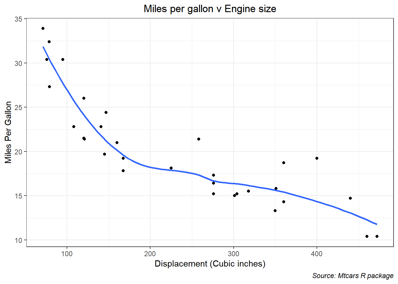
I used the default method in R to fit a smooth line to the data just to see what sort of relationship might be seen here. Clearly it is non-linear (maybe log?). That implies it might not be the best plan to fit a linear regression. But we’re going to anyway because we want to see gradient descent in action.
The following code initializes my gradient descent. Notice I took my first guess at the betas. This is another of those small differences between econometrics and ML. In econometrics we would look at this problem and say “I want a linear model, then I’ll attempt to explain the size and direction of the betas.”
In contrast, for ML we say “we want the machine to learn how to predict this data, so we’ll make a first guess using our human power and give that to the machine to refine.” I used some eye-balling and simple algebra to guess that the \(y\) intercept is around 35 and the slope I randomly set at -9.
obs <- length(data$mpg)

small_x <- matrix(data$disp)

x_dumb <- cbind(rep(1, obs), small_x)
y_dumb <- data$mpg
learn_rate <- 0.0000001
b_0first <- 35
b_1first <- -9
Now to run the gradient descent, I ran this 4 times (3 plus the initial) because that’s enough to get a sense of what’s happening.
## initial state
beta_first <- rbind(b_0first, b_1first)
cost0 <- sum((x_dumb%*%beta_first - y_dumb)^2)/(2*obs)
## first iteration
costderiv <- (1/obs)*(t(x_dumb)%*%(x_dumb%*%beta_first - y_dumb))
beta_snd <- beta_first - learn_rate*costderiv
cost1 <- sum((x_dumb%*%beta_snd - y_dumb)^2)/(2*obs)
## second iteration
costderiv2 <- (1/obs)*(t(x_dumb)%*%(x_dumb%*%beta_snd - y_dumb))
beta_3rd <- beta_snd -learn_rate*costderiv2
cost2 <- sum((x_dumb%*%beta_3rd - y_dumb)^2)/(2*obs)
## third iteration
costderiv3 <- (1/obs)*(t(x_dumb)%*%(x_dumb%*%beta_3rd - y_dumb))
beta_4th <- beta_3rd -learn_rate*costderiv3
cost3 <- sum((x_dumb%*%beta_4th - y_dumb)^2)/(2*obs)
## stack the costs into a vector
cost_vec <- c(cost0, cost1, cost2, cost3)
beta0_vec <- c(beta_first[1], beta_snd[1], beta_3rd[1], beta_4th[1])
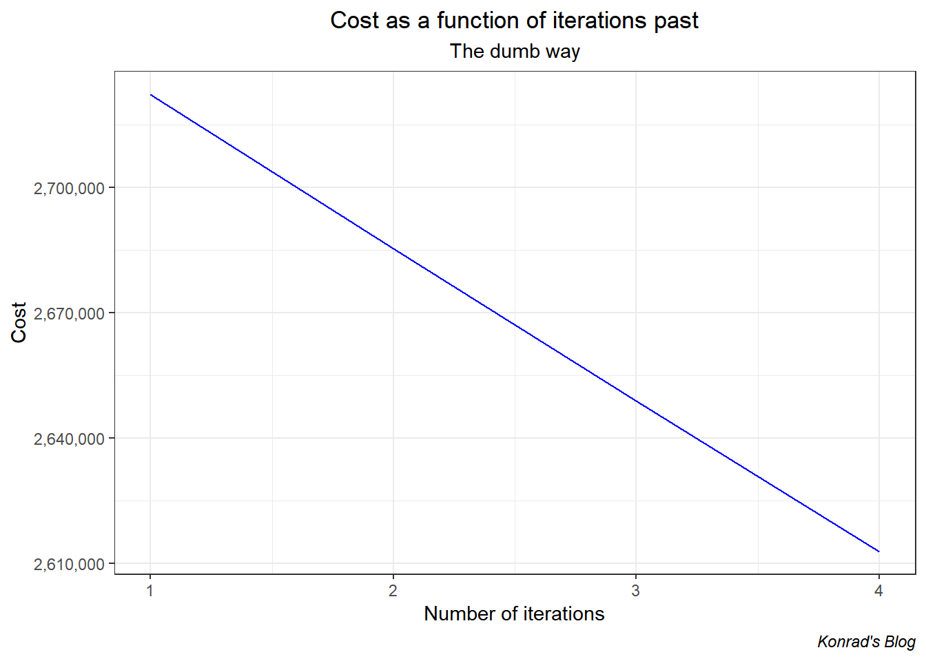
beta1_vec <- c(beta_first[2], beta_snd[2], beta_3rd[2], beta_4th[2])And below I graph the cost function (yay it’s decreasing).
And finally, let’s just see what the estimates for the slope are.
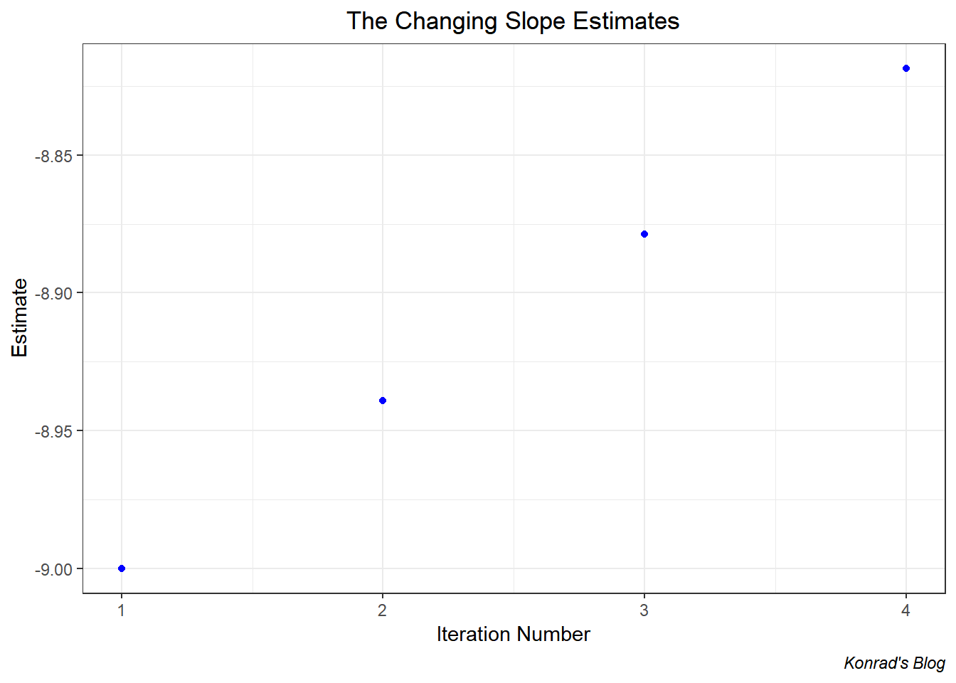
The slope estimate starts at -9 and pretty quickly jumps up to over -7.5. This is a good sign it tells me I set the slope estimate far too large (in absolute terms) in the beginning.
So that’s the kludge way to implement gradient descent. You can, in theory, sit down for a weekend and type out 1,000 iterations of that and you’d have your results. But why do that when computers exist that can iterate over things.
In the next blog post I’ll explain my version of a vectorised gradient descent function that tracks the cost at each iteration. This allows us to plot the “cost curve” and see if it is decreasing with each iteration.
