Gradient Descent The Smart Way
Gradient Descent, the smart way
In this blog post I want to document my version of a gradient descent algorithm. First we’ll take a look at the data, and fit a linear model to it to understand what we’re trying to get to. Remember we can solve for the \(\hat{\beta}\) matrix either through assuming the \(\epsilon\) are IID and solve for a closed form solution using a Maximum Likelihood Estimator (this is the Econometrics way). OR, we can design an algorithm that gets closer and closer to the closed form solution at each iteration. This is the Machine Learning way.
The Machine Learning and the Econometrics way are both getting to the same solution in the case of linear regression.
The dataset I’m using is some made up data used in the Machine Learning course on Coursera.
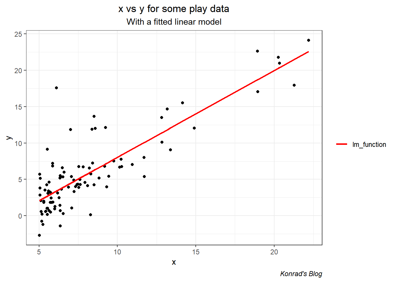
So let’s see what we’re dealing with. Below I plot the data as points, and fit a linear model using R’s lm() function. R’s lm() function estimates that \[\mathbf{\hat{\beta}} = \left[\begin{array} {r} -3.9 \\ 1.19 \\ \end{array}\right]\]
The predicted values form the lm() function are shown in red.
Now on to my Gradient Descent algorithm.
# set the hyper-parameters

learn <- 0.01
numits <- 2000
n <- length(y)

# initialize beta

beta <- matrix(0, 2, 1)

# we also want a vector that stores the cost at each iteration (so we can graph it later)
cost_history <- rep(0, numits)

# we want a function to compute the cost, and a variable to store it

costfun <- function(x, y, beta){
  h <- x%*%beta
  error <- h - y
  cost_at_beta <-  sum((error)^2)/(2*n)
  return(cost_at_beta)
}
Now we want the actual gradient descent. This algorithm needs to take x, y, beta, the learning rate, and the number of iterations. Then, at ach iteration update the beta using the “update amount” it found from the derivative of the cost function evaluated at the previous beta. Inside this function there will be a routine that stores the cost at each iteration in the vector we created during the initialization step. This routine uses the function I made called costfun.
Finally, we want to be able to look at the estimated beta AND the estimated costs so we need to make a list of those two vectors
gradient_desc <- function(x, y, beta, learn, numits){

  for(i in 1:numits) {
  h <- x%*%beta
  error <- h - y
  beta_change <- learn*(t(x)%*%(error))/(n)
    beta <- beta - beta_change
    cost_history[i] <- costfun(x, y, beta)
  }
  results <- list(beta, cost_history)
  return(results)
}

# and store everything (I did this in a weird way, you can also put these inside the functions, but this way is intuitive to me)

results <- gradient_desc(x, y, beta, learn, numits)
beta <- results[[1]]
cost_history <- results[[2]]
Now let’s graph the cost as a function of the number of iterations. We do this to test if our cost function is well behaved and as an idiot check. What we want is a declining function.
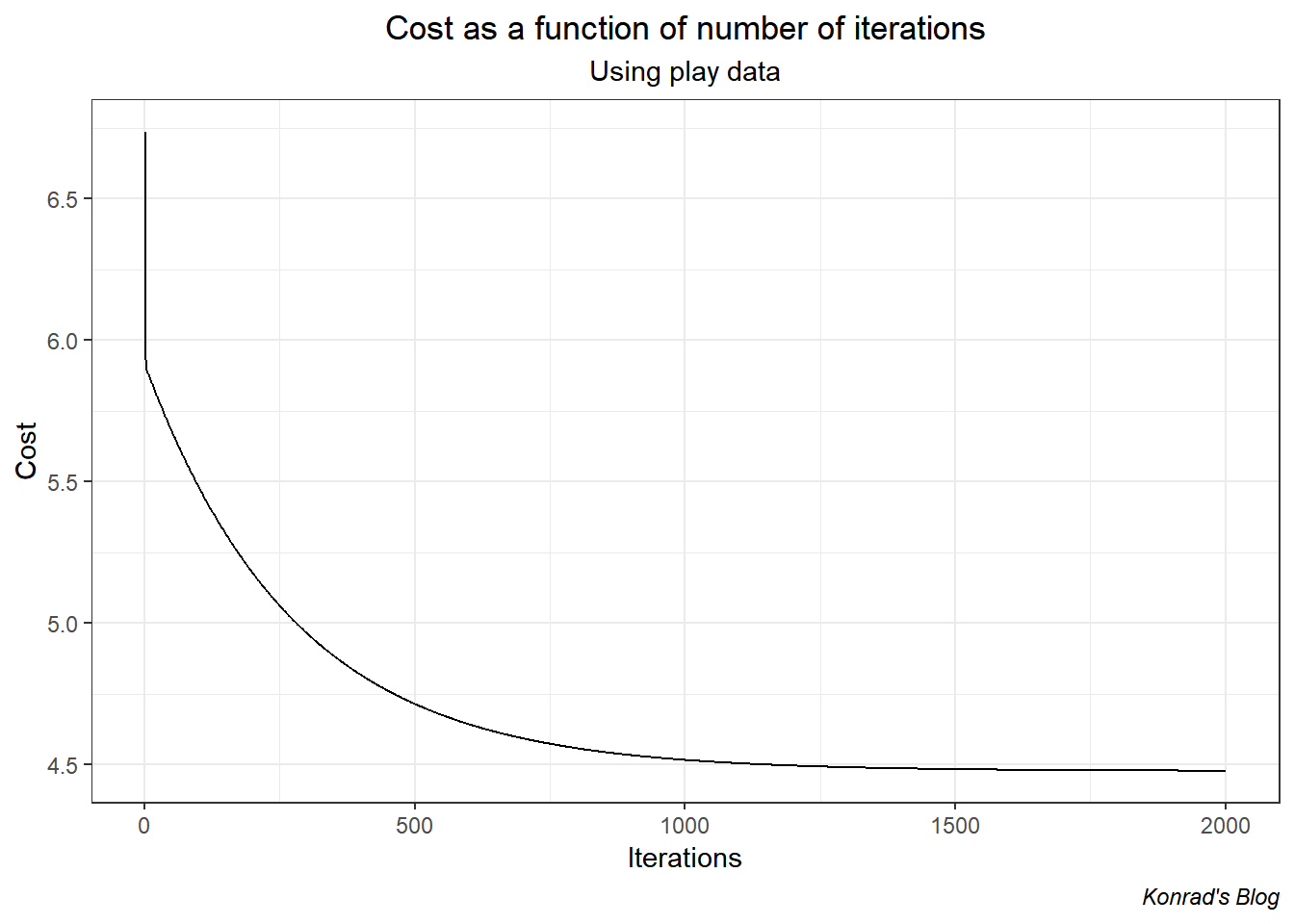
Cool, the function sharply declines and then levels off. This shape implies the cost function is well behaved and the Gradient Descent algorithm has been implemented properly.
Let’s now graph the data, the fitted values from lm(), and the fitted values from my Gradient Descent algorithm.
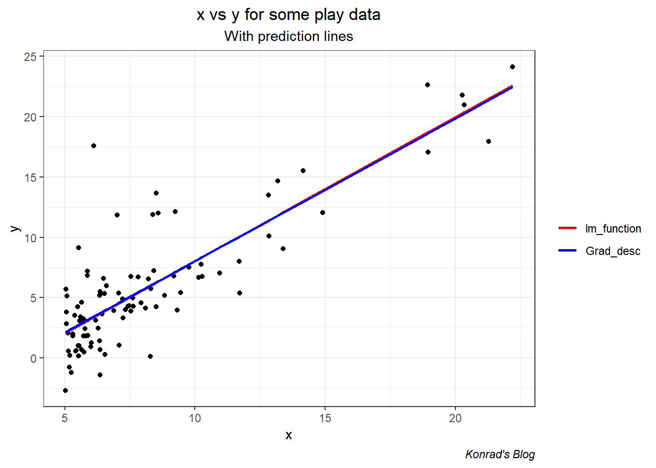
Excellent. The values are VERY close (-3.79 and 1.18, compared to lm()’s -3.9 and 1.19). This is expected as explained before: in the linear regression context Gradient Descent will approximate the linear regression. Once we start considering other model types (like decision trees, neural networks, etc.) the lm() function will fall over.
And with that, we’re done.
