Logistic Regression with gradient descent

In this post we’re looking at my second favourite machine learning algorithm - logistic regression. This algorithm is incredibly useful: Imagine you’re a central planner and you have a dataset of, let’s say, 18 - 24 year olds. Prior to gathering this data you decided you would randomly allocate driver’s licences to half of these 18 - 24 year olds without reuiring them to sit their formal tests. And now you want to assess whether you doing so had any effect on their labour market outcomes (let’s just say employment).

We have a few options - we can fit a linear model (like the previous blog post) with a binary dependent variable \(y = \{unemployed, employed\} = \{0,1\}\) and do a pretty standard test for statistical signifance on the coefficient for licence \(\beta_{licence}\). But what if we care not just about the statistical significance but about the numeric significance. I.e what if we want to know “how much mor elikely is an 18 - 24 year old to be employed given the treatment of being assigned a driver’s licence?”. For that we use a logistic regression.

We do have to be careful that we don’t interpret this as causality though. That is a seperate statistical and philosophical consideration.

In machine learning, because the goal is usually different than econometrics, we might use a logistic regression to decide whether, given some information about a thing, it belongs in one group or another. This is called classification.

Maybe, as in the previous example we have a dataset of 18 - 24 year olds, and their labour market status (employed or not) and we want to predict whether they have their driver licence. This might be useful in the beginning of such an exercise for the central planner to understand how many driver licences need to be allocated. It’s also important for a related issue - matching. This is a process where we try to find people in a dataset who had a “close enough” probability of being treate dor not. This effectively creates an imaginary random trial experiment. In the current examplew e have some made up data and I will show you how to run a gradient descent algorithm to get a solution for a logistic regression problem. I will then show you how to do so using the glm() R function with a pretty graphic.

In the last post I found a solution to a linear regression problem and my estimate of \(\beta\) was almost exactly the same as the lm() function. This post is more of the same. Slight difference but we can get arbitrarily close using more iterations or different learning rates. It helps substantially that I scaled the data. This helps because it means the cost function isn’t “stretched” in a particular direction to some silly degree. Which makes the algorithm faster.

This brings up the question of why you would use gradient descent and not just use closed form methods. Closed form methods take more machine resource and time. So, for example, if you have a phone app that classifies dogs in real time using the camera you can’t be waiting for the processor to calculate the closed form solution using a similar method to glm().

# scale all the data (we need this for later)

training_set[-3] = scale(training_set[-3])
test_set[-3] = scale(test_set[-3])

# make the x and y vars

eX_train <- as.matrix(cbind(1, training_set[1:2]))
wai_train <- as.matrix(training_set[3])

eX_test <- as.matrix(cbind(1, test_set[1:2]))
wai_test <- as.matrix(test_set[3])

#set parameters

learn <- 0.1
numits <- 20000
n <- length(wai_train)

# initialize beta
beta <- matrix(0, 3, 1)

for(i in 1:numits) { 
    h <- sigmoid(eX_train%*%beta)
    error <- h - wai_train
    beta_change <- learn*(1/n)*(t(eX_train)%*%(error))
    beta <- beta - beta_change
    
}



predicted_wai = sigmoid(eX_test%*%beta)

glm() version with pretty graphics

colnames(ex2data1) <- c("var1", "var2", "why")

split = sample.split(ex2data1$why, SplitRatio = 0.75)
training_set = subset(ex2data1, split == TRUE)
test_set = subset(ex2data1, split == FALSE)

training_set[-3] = scale(training_set[-3])
test_set[-3] = scale(test_set[-3])

logistic <-  glm(formula = why ~ .,
                 family = binomial,
                 data = training_set)

prob_pred = predict(logistic, type = 'response', newdata = test_set[-3])
y_pred = ifelse(prob_pred > 0.5, 1, 0)

set = test_set
X1 = seq(min(set[, 1]) - 1, max(set[, 1]) + 1, by = 0.01)
X2 = seq(min(set[, 2]) - 1, max(set[, 2]) + 1, by = 0.01)
grid_set = expand.grid(X1, X2)
colnames(grid_set) = c('var1', 'var2')
prob_set = predict(logistic, type = 'response', newdata = grid_set)
y_grid = ifelse(prob_set > 0.5, 1, 0)
plot(set[, -3],
     main = 'Logistic Regression',
     xlab = 'var1', ylab = 'var2',
     xlim = range(X1), ylim = range(X2))
contour(X1, X2, matrix(as.numeric(y_grid), length(X1), length(X2)), add = TRUE)
points(grid_set, pch = '.', col = ifelse(y_grid == 1, 'springgreen3', 'tomato'))
points(set, pch = 21, bg = ifelse(set[, 3] == 1, 'green4', 'red3'))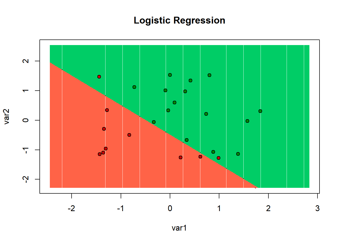

# confusion matrices

cm_GD = table(wai_test, predicted_wai > 0.5)
cm_GLM = table(test_set$why, y_pred > 0.5)

As you can see in the above graphic, there were 2 red points that the algorithm thought were in the green zone. And no green points the algorithm thought were in the red zone.

We can asses show wrong or right out classifiers are by looking at the confusion matrices. These show how many actual 1s were predicted as 1s, and how many actual 0s were predicted as 0s. As well as the combinations where the classifier got it wrong.

Basically you want the numbers on the diagonal (from left top corner) to be big and the other numbers to be small. We observe this result which is encouraging. Both the glm() classifier and my classifier trained via gradient descent display good results.

cm_GD

##         
## wai_test FALSE TRUE
##        0     8    2
##        1     1   14

cm_GLM

##    
##     FALSE TRUE
##   0     8    2
##   1     0   15